![]()
![]()
![]()
![]()
![]()
![]()
Input Sensors: 7x Sonar Sensors, 4 x IR Range Finders, 1x Gyro, 2x Wheel Click Sensors, Active Behaviour
For the robot to be useful in the real world it requires some sort of world representation to determine where it is, where it's been, where is going and help it work out how it's going to get there.
To achieve these the HCS builds a map based upon the the probability of there being free space or occupied space within a the area the robot has roamed.
A sonar's beam is not just a straight line from the point of origin to the obstacle and back again. The sonar energy spreads out in a cone from the sonar. The further away from the centre the When creating a map this needs to be modelled. The sonar is modelled as follows:
The field of view, termed β.
The half angle of the cone, R
The maximum range it can detect.
The sonar range is split into three regions. The regions determine whether the probability of a cell being occupied or unoccupied can ever reach 1.0, that is whether there is any possible doubt as to the state of the cell.
Cells in Region 1 are the cells which are probably occupied. These cells can never reach 1.0 certainty.
Cells in Region 2 are the cells which are probably empty. These can become attain a value of 1.0 certainty of the cells state.
Cells in Region 3 are un affected by the sonar beam.
Figure 1 shows a diagram of the sonar beam.
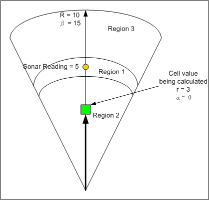
Figure 1
For each cell which falls within the sonar beam the probability that a sonar reading is detecting occupied or unoccupied space is captured by the following equations:
For Region 1:
P(Occupied) = (((R - r) + (β - α)) / 2) * MaxOccupied
P(Unoccupied) = 1.0 - P(Occupied)
For Region 2:
P(Occupied) = ((R - r) + (β - α)) / 2)
P(Unoccupied) = 1.0 - P(Occupied)
These calculations give probabilities of the form P(s | H), specifically P(s | Occupied ) and P (s | Empty). Which means the probability that H has occurred given the sensor reading s.
To determine the difference between Region 1 and Region 2 a tolerance is used. This is the resolution of the sonar - I used a value of 8.
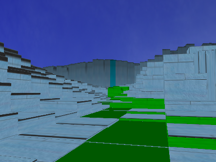
Figure 2
Figure 2 shows the OpenGL model of a single sonar beam. The green line depicts the ideal line of travel, the end of which is coloured differently (Teal colour) to depict the change in region from Region 1 to Region 2. The model shows that as the beam travels further away from the robot, and the further off centre the beam becomes, the certainty that a particular cell is occupied decreases and similarly the certainty that a cell is occupied increases (i.e. the cell height increases, to model the concept of an object)

Figure 3
Figure 3, above shows a couple of modelled sonar beams. The ideal beam is identified by the light green line (Region 1), which changed colour into a teal colour (when in Region 2). The image also shows how the uncertainty of the area being free space decreases (The "land" is less flat) the further away from the robot and the further off centre the beam becomes.
The occupancy grid is designed to grow dynamically with the area that has been explored by the robot, therefore there is not theoretical limit on the range of the robot. In practice this is more like 50sq meters before inaccuracies creep in which can corrupt the map.
As the robot sends data back to the host all the ranging finding data is applied to the map and it works out which cells to update depending on the robots orientation and position in space.
Given the equations for occupied and empty space above, there needs to be away to integrating the data into the overall map (Occupancy grid). To achieve this the map is updated using Bayes' rule.
Bayesian Rule:
P(H|s) = ( P(s|H) P(H) ) / ( P(s|H) P(H) + P(s|¬H) P(¬H) )
Each time a new cell is created its initial value is set to 0.5 for both the occupied and Empty space. Over time the Bayesian updates will modify this to either become strongly occupied or empty.
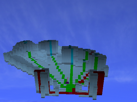
Figure 4
Below, figure 5, shows the robots view/model of a room (The actual lay out of which is shown in figure 6). The occupancy grid nicely models the free space (Light and low lying cells) with that of occupied space (High and darker cells). Some of the obstacles in the room were producing poor sonar reflections, therefore this gets modelled as a some where in-between the high and flat cells, that is the map is unsure. Comparing the occupancy grid with the real room there is a very good correlation between the shape of the free space in the model with that in the real room.
The red lines are only active when the IRRFs are with in their specified limits; that is when they are between 10cm and 100cm and their respective sonar is reading a distance within the the Object Near range.
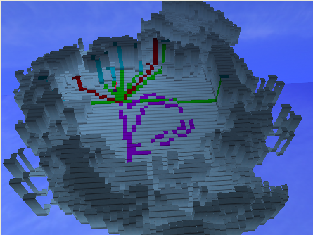
Figure 5

Figure 6
Code below is for determining and updating a cell in the occupancy grid.
// Determine the probability that a cell is
occupied.
double CMapEnvironment::ComputeCellRegion_P( double MaxSonarDistance,
double SonarMeasuredReading,
double HalfConeAngle,
double CellDistance,
double CellAngle)
{
// P(Si|C) i.e The probability that C is occupied, given
sensor reading Si
const double M = 0.98;
double CalcVal = 0.0;
double P1, P2;
P1 = (static_cast<double>(MaxSonarDistance) - static_cast<double>
(CellDistance))/static_cast<double>(MaxSonarDistance);
P2 = (HalfConeAngle - CellAngle )/ HalfConeAngle;
CalcVal = (P1 + P2)/2;
return CalcVal;
}
// Using Axiom equations above update the cell according to Bayes Rule
double CMapEnvironment::BayesianUpdate(GridCell * CellToUpdate)
{
double BayesianValue = 0.0;
double PriorOccupancyValue = CellToUpdate->OccupancyProbability;
double PriorEmptyValue = CellToUpdate->EmptyProbability;
double MaxOccupied = 0.98;
double OccupancyValue = 0.0;
double EmptyValue = 0.0;
// P(Si|C) P(C)
// ---------------------------
// P(Si|C)P(C) + P(Si|¬C)P(¬C)
double P = ComputeCellRegion_P( CellToUpdate->MaxSonarDistance,
CellToUpdate->MeasuredSonarDistance,
CellToUpdate->BetaHalfConeAngle,
CellToUpdate->GridCellDistance,
CellToUpdate->AlphaAngleOffset);
// If we're in region 1 then it is most likey that the cell
will be occupied. Further more
// it cannot become 1.0, hence the (* MaxOccupied)
calculation.
if(CellToUpdate->CellsRegion == Region1)
{
OccupancyValue = P * MaxOccupied;
EmptyValue = 1.0 - OccupancyValue;
}
else
{
EmptyValue = P;
OccupancyValue = 1.0 - EmptyValue;
}
CellToUpdate->OccupancyProbability = ( (OccupancyValue*PriorOccupancyValue)/(
(OccupancyValue*PriorOccupancyValue) + (EmptyValue*PriorEmptyValue) ) );
CellToUpdate->EmptyProbability = ( (EmptyValue*PriorEmptyValue)/(
(EmptyValue*PriorEmptyValue) + (OccupancyValue*PriorOccupancyValue) ) );
return BayesianValue;
}